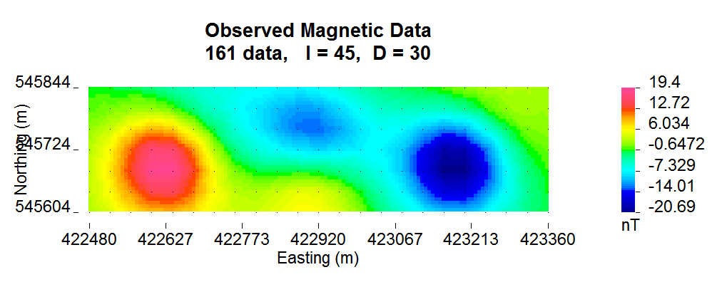
5. Examples
In this section, we present a simple synthetic example to illustrate forward modelling and inversion of magnetic vector models. For more in-depth training material, please visit our AtoZ example .
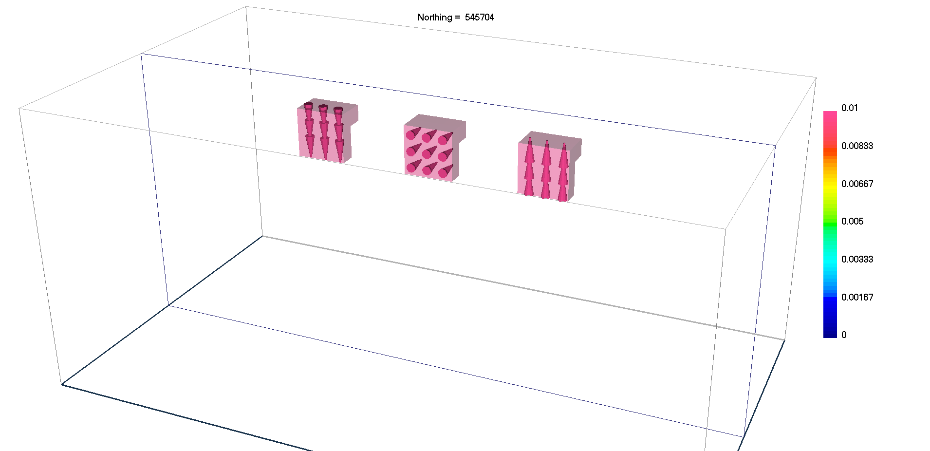
The example is made up of three magnetic block, 120 m in side length, placed 85 meters below a grid of observation points. The blocks are magnetized along different directions, indicating the effects of remanent magnetization are large.
The example, including the model and simulated data, can be downloaded here.
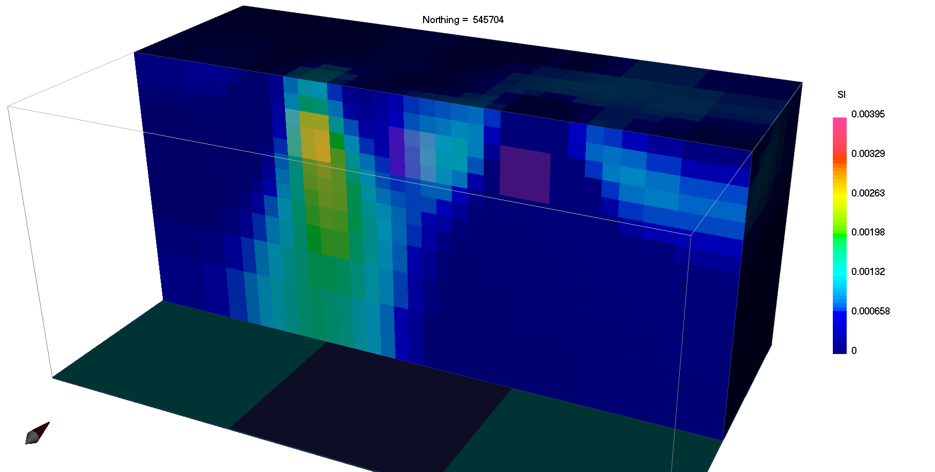
5.1. Susceptibility Inversion
To demonstrate the importance of accounting for remanence, we first assume all magnetization is induced and invert the data using the MAG3D inversion program. Below we see that the final magnetic susceptibility model clearly fails to recover the shape and location of the three magnetic blocks.
5.2. Magnetic Vector Inversion
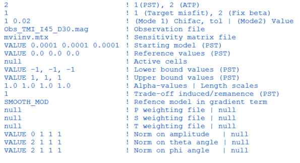
In order to properly account for arbitrary orientations of magnetization, the data are re-inverted with the MVI algorithm using the input file shown below. Plotted are a smooth solution recovered using the Cartesian formulation and a sparse solution recovered using the Spherical formulation
Comparing the results we note that:
The smooth solution (MVI-Cartesian) imaged all three blocks at the correct locations and the magnetization directions at the center of each block are well recovered. The center block is much more difficult to identify.
The sparse solution (MVI-Spherical) greatly simplified the magnetization model and highlighted the presence of the center block anomaly.